Similarity-driven Brain

December 22, 2019 | 40 Minute Read

Human brain has so various functions that we couldn’t solve the whole mystery yet. In order to understand the function of brain or its nature per se, people have suggested and developed many computational models and explained our brain. This is based on the basic assumption that human brain internally computes or handles symbols or representations of external worlds. The Artificial Neural Network (ANN) is a way of doing that and it has many industrial applications in wide ranges, as well as in brain research area. The ANN, however, is successful only in small problem-specific areas such as pattern recognition, classification, associated memory, etc. In this work, I explored the nature of brain more deeply and made a general assumption that human brain always seeks similarity among external stimulus. On this assumption, I suggest a general neural network model, which is more similar to real neurons in brain than other ANNs, and is suitable for large networks due to its scale-free feature. I also suggest that basic functions, such as logical operation and classification, can also be implemented by seeking similarity among stimulus. The suggested model is simulated in Matlab® environment and shows expected behaviors, though there still remain some issues to generalize it.

INTRODUCTION

The Artificial Neural Network, which basically takes a bottom-up modeling method from a single neuron to the whole brain, has developed many variants depending on its application, since the Perceptron by Rosenblatt appears for the first time in 1957 (Kim 1995). It has powerful advantages in implementing artificial intelligence compared with the symbolic approaches despite that the trained neural network can’t give any plausible explanation of behavior at neuronal level. In this work, I propose a similarity-driven neuronal model, which can be a basic building block to constitute complex neural networks. The proposed model adopts various intuitions from real brain architecture and other network structures, and thus shows a possibility to be generalized by the mechanism of seeking similarity among stimulus.

Scopes of the Work I have three objectives in this work, as shown in the following.

• Brief review of previous Artificial Neural Networks
• Study of the basic neuronal architecture and its implications
• Suggestion of new neural network and verification of its operations

This is a tentative work, and therefore various applications using the proposed model are not tested here. But, the crucial idea of this model is fully described and I guess that it is possible to develop any specific application based on this model.

Neural Networks Revisited The Artificial Neural Network (ANN) is inspired by biological neural networks in brain, and has many advantages. Unlike conventional symbolic approaches, which operate well only in their prescribed domains, the ANN shows no brittleness outside its domain, as a result, the graceful degradation outside its domain is a major feature of ANN. Then, let’s see in brief what is different from conventional approach, e.g. Von Neumann architecture or modern parallel computers (Jain et al. 1996).

• Massive parallelism
• Distributed representation and computation
• Learning ability
• Generalization ability
• Adaptivity
• Inherent contextual information processing
• Fault tolerance
• Low energy consumption

Firstly, the ANN uses massive parallelism in computation. Although modern parallel computers also use parallelism in computation, their parallelism is only for speeding the whole operations. That is, there still exists central processor (or processors in case of multi-processor system) to control the overall system. So, the whole operations are controlled sequentially by the processor. Unlike this, the ANN has no central processor and functions of the ANN are determined by the connectivity of ANN itself. Owing to this feature, the ANN has distributed representation and computation. It means that the ANN doesn’t have any symbol representation of single node. All data or functions are represented with a lot of nodes or neurons. Thus, the ANN is more robust than symbolic approach. In representation of a single node, in case that a fault occurs at any node, the node output is fully corrupted and may cause a severe failure of the whole operation. However, in distributed representation, a failure at one of many distributed patterns is not critical to the whole operation and thus the ANN has fault tolerance feature. Another advantage to note in the ANN is learning ability. In fact, the learning ability is an essential feature of artificial intelligence, and is important when implementing all ANN systems. At the same time, learning is not an easy process and determines the performance of the ANN. The learning ability is consistent with the adaptivity feature. If a system has a learning ability, it is also believed that it is likely to adapt to new environment or stimulus. The more the ANN adapts to new environment, the more the ANN is generalized. In other words, the generalization ability comes from many adaptations. After the ANN is trained through given many examples, it is generalized, i.e. it can solve many other problems not given in the training set. For example, consider the curve fitting problems. The trained ANN can predict new data set on basis of the training data set. Like this, the structure of ANN is closely related with the training set. This gives rise to another feature of ANN, i.e. inherent contextual information processing. All ANNs have contextual information of processing, which is given by training. The information is represented as a structure or connectivity of ANN. Last but not least, the ANN shows low power consumption. This is not crucial in case of modeling and studying brain functions. The industrial applications, however, need to consume power as low as possible. With respect to power consumption, the ANN is superior to modern computers, because it doesn’t have complex centers or functional modules to control.

Which problems can the ANN solve? There are many problems effectively solved by the ANN, which are interesting to computer scientists and engineers. Some of them are shown in Figure1 (Jain et al 1996). Pattern Classification The ANN can classify an input pattern, e.g. handwritten letter or visual scene, which is represented by a feature vector to one of many pre-specified classes. It also has many application areas such as speech recognition, character recognition, EEG waveform classification, etc. Clustering/Categorization Unlike pattern classification, clustering doesn’t have supervisor. That means, in clustering or categorization, there are no training data with known class labels. A clustering algorithm seeks any similarity between the patterns and places similar patterns in same cluster. The typical applications of clustering are data mining and data compression.

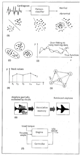
Function Approximation This is a problem like a well-known curve fitting. For example, for input patterns of 2-dimensional data (x, y), we have an unknown function y=f(x), which generates the given data set. The task of this problem is to find an estimate, say ŷ, of unknown. Most scientific experiments require this kind of approximation for the results to make a plausible model. Prediction/Forecasting Prediction or Forecasting is done in a time sequence of data. The task is to predict the sample data at some future time tn+1, with a time sequence t1, t2, …, tn. Prediction mainly affects human decision-making in business, science, and engineering. The above example of stock market in Figure1 is a typical application of this problem.

Optimization Almost all application areas have an optimization problem. The goal of an optimization algorithm is to find a solution satisfying a set of constraints such that an objective function is maximized or minimized. The well-known Traveling Salesman Problem (TSP), an NP-complete problem, is also a classic example. Content-addressable memory This isn’t an easy problem for von Neumann model of computation, which uses exact address to access a memory data. If missing even one bit of its address, it can’t retrieve the right content. Content-addressable memory or associative memory, as the name implies, can be accessed by their contents per se. Thus, the memory contents can be recalled even by a partial input or distorted content. Associative memory is extremely desirable in noisy systems. Control In a dynamic system, defined by an input x(t) and an output y(t), the goal is to generate a control input x(t) so that the system can follow a desired trajectory determined by the reference model. The typical example is an idle-speed control of an engine.

As we have seen so far, the ANN makes it easier to solve the above problems effectively. But, if an ANN is trained to solve one specific problem, it’s useful to solve others one no more. Moreover, the architecture of ANN to solve one problem is not suitable for other one, e.g. the ANNs for clustering/categorization and content-addressable memory have different structures so that they aren’t interchangeable each other. Therefore, the ANNs have ever developed problem-specific or domain-specific neural networks. In the following paragraph, I’ll show simple classification of the ANN. Simple classification of the ANN Though there’re many variants of ANN, they can be divided into two classes depending on whether recurrent or feedback path exist or not. In Figure2, taxonomy of the ANN is shown. For Feed-forward networks, perceptron and radial basis function network are shown here. The Single-layer Perceptron is developed by F. Rosenblatt from the first neural network model, McCuloch-Pitts neuron, on the basis of Hebbian Learning rule. It has basic computation unit, TLU (Threshold Logic Unit), which is a special type of McCuloch-Pitts neuron. Rosenblatt proposed a single-layer perceptron as a general intelligent system irrespective of specific biological system.

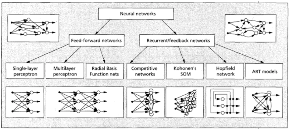
It consists of sensor input, response output, and neuronal layer. The output function is nonlinear and has one or zero after compared with its threshold. The learning rule adjusts the weight values by the difference between output value and expected value. The Multilayer Perceptron has an intermediate layer, hidden layer, between an input layer and an output layer. However, there is no direct connection from input to output. It has nonlinear characteristics for input and output, and due to this nonlinearity, multilayer perceptron enhanced ability of networks largely. Actually, a multilayer perceptron can solve the exclusive-OR problem, which can’t be solved in a single-layer perceptron. It uses a back-propagation algorithm to adjust the weight values and train the network, where it back-propagates the errors between the output and expected values, and minimizes total amount of errors by gradient descent method, which is called generalized delta rule. The Radial Basis Function (RBF) network also has two layers and is a special class of multilayer feedforward networks. Each unit in the hidden layer employs a radial basis function, such as a Gaussian kernel, as the activation function. The RBF network learns both positions and widths of these kernels by training. Each output unit implements a linear combination of these radial basis functions. The ANNs explained up to now only have forward paths, that is, all output is determined by only input data. But, we can annotate more complex features on ANN by adding recurrent path. The Competitive Network is one of such networks. Unlike hebbian learning, which has multiple output units, competitive learning output units compete among themselves for activation. As a result, only one output unit is active at any given time, which is known as winner-take-all. Competitive network often clusters or categorizes the input data. That is, similar patterns are grouped by the network and represented by a single unit. Thus, even though there is no supervisor to teach how to classify, competitive network can do it automatically based on data correlations. Kohohen’s SOM (Self-Organzing Map) is a special type of competitive network that defines a spatial neighborhood for each output unit. By do that, SOM has the desirable property of topology preservation, which is often observed in highly developed animal brains. It basically consists of a two-dimensional array of units, each connected to all n input nodes. Each neuron computes the Euclidean distance between the input vector x and the stored weight vector w. Kohohen’s SOM has been successfully applied in the areas of speech recognition, image processing, robotics, etc. In a way, Hopfield network uses an energy function as a tool for designing recurrent networks and for understanding their dynamic behavior. Hopfield’s formulation makes explicit the principle of storing information as dynamically stable attractors and popularized the use of recurrent networks for associative memory and for solving combinatorial optimization problems. The patterns stored these network attractors can be used as an associative memory, i.e. any pattern present in attraction of a stored pattern can be used as an index to retrieve it. Usually, an associative memory operates in two phases: storage and retrieval. While new knowledge is learned and stored in storage phase, in retrieval phase, the existing knowledge is recalled. But then, how can we learn new things while retaining stability of existing knowledge? This is stability-plasticity dilemma. Carpenter and Grossberg’s Adaptive Resonance Theory (ART) model is developed to overcome this dilemma. The ART model has extra-outputs which are not used until deemed necessary. A unit is said to be committed (uncommitted) if it is (is not) being used. Learning algorithm updates the stored prototypes of category only if the input is sufficiently similar to them. That is, ART has an ability to estimate how much different the input is from the stored data pattern before updating the network. In addition to above networks, there are many variants of ANNs. All networks have their own learning algorithms and structures depending on their application. Also, they are inspired by hebbian learning rule biologically. Drawbacks of previous ANNs Although ANNs are useful for many applications, they still have some drawbacks. First of all, the training a network is not easy and learning needs much time. Especially, in order to simulate various functions of brain and apply to industrial systems, they have no choice but to have more complex learning algorithms according to the structure they have. Besides, the learning process is not similar to real brain environment in some senses. Also, they have a special structure to be optimized for a specific application. Thus, one model cannot be applied to another situation generally. Human brain has various neurons morphologically, of course, but we need general model to show how basic neuron works. This is very important in that it’s very helpful to have a hierarchical model to explain brain because human brain is too complex to get the whole process for now. That is, we need a basic building block model to constitute the whole brain or at least a small functional circuit. With all these reasons, current models are little helpful to understand human brain. The main purpose we develop ANNs is to understand human brain more deeply and discover the mystery of intelligence and mind, as well as practical usage such as industrial application. In this sense, there are many rooms to enhance or modify current ANNs. I’ll try to make a new model to explain our brain more plausibly and find out its possibility to be used for some application areas.

METHODS

To implement new model for neuron and brain cells, I’ll investigate various facets of our brain until now. From those assumptions, I suggest several applicable hypotheses to make a model in the followings. Large Numbers in Human Brain The Figure3 shows the structure of human brain.

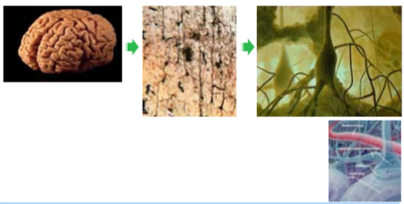
We have huge amounts of neurons in our brain. According to Abeles (1991), the cortical area is about 300,000mm2 in human neocortex when assuming the thickness of cortex is about 3mm. In this area, neuronal density is up to 20,000 ~ 40,000/mm3, and synaptic density is 8×108/mm3. This means that a single neuron has about 20,000 ~ 40,000 synaptic inputs. This is an amazing number considering the input and output of a system, i.e. many connections are inter-wired between neurons. In a way, neuronal composition shows that pyramidal cells are majority (75%) in cortical area, followed by spiny stellate (10%) and inhibitory (15%). The dendritic length of pyramidal cells runs up to 10mm. The pyramidal cells usually accept inputs at cortical layer IV and these signals go to layer II and III, and the final output of these layers are connected to layer VI to be transmitted to other cortical areas. From cortical structure, we see that most synaptic connections are from pyramidal cells and pyramidal cells have many inter-neuron connections at layer II and III. This means that our model should have much more interconnections between neurons than inputs and outputs. Also, although various neurons co-exist in cortical area, the majority of them are pyramidal cells, which means there is a basic building block that has same function.

Scale-Free Network Now, the next problem is how the neurons are connected within cortex. This is an issue about the structure of networks. To solve this issue, I attend to a Scale-Free Network (Barabási 2003a; 2003b). The Figure4 shows a scale-free network.

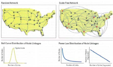
The scale-free network is often observed at various situations, such as internet, skyway, social relationships, etc. It has distinct features that are different from conventional random networks. First of all, the scale-free network has, as the name implies, no scale. That means it is scalable irrespective of network size or connection patterns. Each node in scale-free network can be connected to any other nodes freely. There are no scales or restrictions. The Figure5 shows the birth of a scale-free network (SFN).

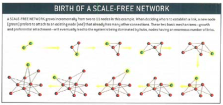
The scale-free feature of SFN lets an interesting node, Hub, emerge. The Hub is a node which has especially many connections from other nodes. There are huge traffics at hub, compared with normal nodes, i.e. the rich gets richer. The existence of hub might be good or not. The hub is more important than other nodes because of its heavy traffic. Thus, if damaged to hub, SFN will lose many connections and information. This is similar to an internet, which is vulnerable to coordinate attack. But, still, it is powerful in that it is robust to accidental failure at normal nodes. I think that our brain is much similar to this network. Human brain shows powerful plasticity when a specific area is damaged, but in some cases, it doesn’t. I guess that brain function can be recovered only if a hub neuron or area is not damaged. Another thing to note here is that SFN has hierarchical clustering. The Figure6 shows a SFN clustering in different hierarchical levels.

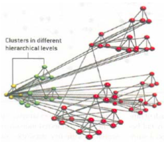
The SFN has basic structure and can span it at various levels. This is also an interesting feature to model our brain. Thus, with all these analyses, I suggest that our brain model may be a scale-free network.

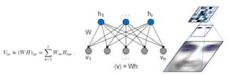
Non-negativity One problem in conventional ANNs is that they have too mathematical or engineered model of computing weights among neurons. That is, to implement negative effect of stimuli, they assume negative weights between neurons. However, in real brain, there is no physical value corresponding to negative weights. Signal transmission in synapse is done by chemical interaction between two neurons, and the transfer is about whether there is an ion flow (positive) or not (zero). To overcome this problem, I introduced the concept of Non-Negative Matrix Factorization (NMF), which is suggested by Lee and Seung (1999). They try to solve a face image recognition problem. In this example, we assume that a face image can be estimated from feature vectors and encoding vectors (Figure7).

This factorization process can be taken differently by algorithms. In case of VQ (Vector Quantization), typical faces in the training set are selected as feature vectors. The encoding process is defined as an estimation of the original face from any typical faces by calculating the difference. PCA (Principal Component Analysis) has similar process except for the feature vectors are not a typical face, but an eigenface. The PCA extracts most integral elements of data by orthogonal transformation. As a result, we have parameterized simple face features.

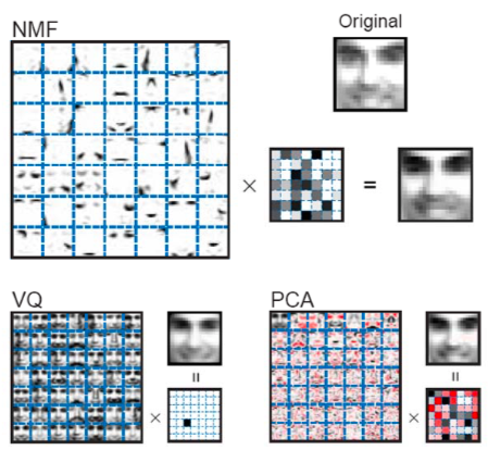
However, unlike two cases, NMF uses parts of the original face as feature vectors. That is, in case of NMF, we can encode the face images with partial information of them. This is a unique feature provided only in NMF. Inspired by this feature, I guess that our neurons have part-based representation and the whole brain can be explained by the parts, i.e. the sum of neurons per se. Also, because firing rate is never negative and synaptic strength does not change sign, weight values to represent the connectivity among neurons should never be negative and learning algorithm must consider this non-negativity. In this respect, the weight values may represent the amount of neurotransmitter between two neurons.

Distributed Representation Distributed representation is a general feature found in most ANNs. But, basically, previous ANNs assume that there is a single output node indicating the computation result. For example, in Kohonen’s SOM, only the winner neuron is activated. But, I think that the output is also distributed in human brain, as well as the computation process.

In Figure9, the neurons in visual cortex fires at each face stimuli, where the output of each neuron is collected and becomes patterns for input stimulus. In other words, all neurons equally contribute to discriminate the face. This implies that ANN should have distributed output nodes to represent neural state. The distributed representation is beneficial even in view of information processing. Distributed representation increases encoding capacity and is robust to simple damages. Besides, since there is evidence that our neurons have multi-modal characteristics in a single neuron, e.g. columnar structure with ocular dominance and orientation selectivity, information of patterns is natural consequence. Then, how distributed are neurons? The plausible idea here is correlation between each neurons based on similarity. The neuronal output, for example, may be encoded based on whether the input face stimulus is similar or not. On this assumption, I’ll try to explain neuronal model in the following sections.

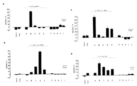
Sparse Representation Conceptually, sparsity corresponds to systems which are loosely coupled. In a sparse system, there is a line of connections from one to another. By contrast, in a dense system, all possible connections exist among every node. Sparsity is a useful concept in real brain modeling. Let’s see the following Figure10.

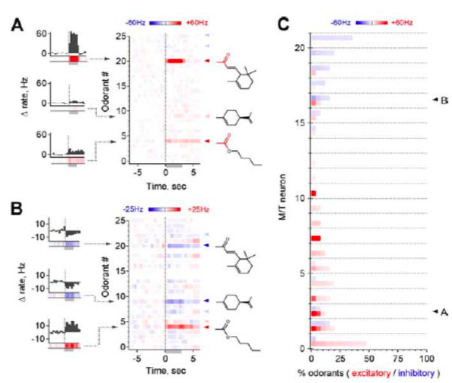
The result shows that when activated by odorants, M/T cells are selective, with neurons responding robustly, sensitively, and reliably to only a highly restricted subset of stimuli. Also, for multiple odorants, a single neuron shared structural similarity in common. This suggests that individual M/T neurons encode specific odorant attributes shared by only a small fraction of compounds and narrowly tuned to a particular stimulus characteristic. Shortly speaking, M/T cells are systematically distributed throughout chemical space and use sparse and selective odor coding scheme. This means that there are highly concentrated connections among neurons, say Hubs, normal neurons except hubs are connected sparsely, on the contrary. Therefore, our new model should have sparse coding with respect to hubs.

Long-Term Potentiation (LTP) Mechanism Long-Term Potentiation is a well-known phenomenon which is regarded as a synaptic plasticity related to memory. Until now, LTP(Long-Term Depression (LTD) is similar to LTP in terms of its process. The difference between those two terms is only the direction of potential change.) is thought to be a static process generated in an over-stressed neuron by same stimulus, i.e. repetitive stimulus can change the neuronal state and sensitize it for input. But, recently, there was another report for LTP mechanism in barrel cortex of mice (Clem et al. 2008). The following Figure11 shows the result.

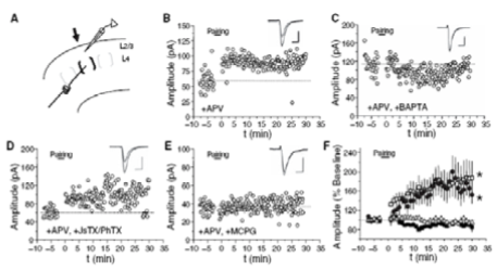
They removed all whiskers of mice except for one target whisker and stimulated it repetitively until it shows LTP phenomenon. Generally, LTP is believed to occur by NMDA receptor (NMDAR). But, they found that there is still LTP after blocking NMDAR by applying APV, which is an antagonist of NMDAR (B). This phenomenon disappeared by inclusion of BAPTA, which is a chelator of Ca2+ (C). That means the LTP without NMDAR needs postsynaptic Ca2+ entry. Now, the puzzle is to find what is related to Ca2+-dependent LTP. Through some trials, they discovered that Ca2+-dependent LTP disappears by including MCPG, which is an antagonist of mGluR (E). That is, mGluR is another source of LTP. If they are right, LTP has two distinct processes: one by NMDAR and the other by mGluR. NMDAR is related with an ionotropic transfer, while mGluR is related with a metabotropic transfer. At first phase of LTP, more direct transfer using NMDAR is activated. But, as LTP is hold for a long time, the indirect transfer using mGluR increases, instead NMDAR activation decreases. In this sense, LTP is a dynamic process, not a static one. To achieve this dynamic process in a neuron, a neuron should monitor itself. In other words, self-monitoring process is needed. Thus, I guess that there is a self-loop in a neuron, which is activated or deactivated by itself. This is another point to note when modeling ANN. Equivalence Network While implementing a distributed representation, a similarity between inputs is considerable. Thus, how to implement similarity on a network is crucial issue. In mathematics, equivalence on a set is defined as the following conditions.

• Transitivity: if A~B,and B~C,then A~C
• Symmetry: if A~B,then B~A
• Reflexivity: A ~ A

In above relation, “A~B” means that A is equivalent to B. I suppose that this relationship can be applied to neuronal connections. Assume that neuronal circuit finds a similarity among inputs. If some inputs activate similar neurons, then they’ll have close relationship. For example, in case of pattern recognition, if two input images are similar, they will activate similar neurons. Thus, if we apply equality on a set to neuronal circuit, the following rules are obtained.

• Transitivity: if A and B neurons are related and B and C neurons are related, then A and C neurons are also related.
• Symmetry: if A is dependent on B, then B is also dependent on A.
• Reflexivity: if A is dependent on itself. These equivalence relations can partition a set into several disjoint subsets, called equivalence classes in Figure12. Thus, I suggest that we can implement a similarity-driven neuronal model using equality. This network can do a natural clustering or classification based on equivalence classes.

Summary of Neuronal Architecture In summary, our new model of neuron should have the following characteristics.

• Large inter-neuron connectivity
• Scale-free network
• Non-negativity
• Distributed representation
• Sparse representation
• Long-term potentiation mechanism
• Equality (Similarity) network With all these results, I make a neuronal model in the RESULTS section.

RESULTS

The proposed model is a neuronal pair that consists of two adjacent synapses(I focused on a synapse, not a soma of neuron that is a place of integrating neurotransmitters and generating spikes. More specifically, a synapse is a dynamic place that network is generated in various form, while a soma is a passive area that receives ion current and discriminates whether to fire or not. Thus, I’ll use a synapse-based model to constitute neuronal circuit.), not neurons. The output is an energy function of such network, which will be one or more. This can be a basic building block of large network of neurons. Depending on a specific application, however, it has a little bit different forms or structures. It’s not an easy work to build a new model and verify its validity. Therefore, in this work, I’ll consider a simple example, logical operation, to verify my idea.

Scale-Free Neural Network Basically, the proposed model is a kind of Scale-Free Networks, which has large inter-neuron connectivity, thus I call it Scale-Free Neural Network (SFNN). The SFNN has a distributed and sparse representation of information, and always seeks a similarity between inputs. As in real brain, there is no negative signal. Also, to achieve neural plasticity, the SFNN adopts new LTP mechanism introduced here. Now, let’s see the basic cell of SFNN.

Basic Cell The following Figure13 shows a basic cell of SFNN.

The main difference between SFNN model and the previous ANN models is that SFNN model uses synapse-based representation. That is, the cell body or soma integrates all inputs from pre-synaptic neurons and generates spikes if the stimuli go beyond the cell firing level. In this sense, all functions of neuron are mainly dependent on synaptic binding. I made a scale-free network model for synaptic binding within a neuron, as well as in a large scale neural network. This network is a form of scale-free network and becomes a building block for complex network. Also, the connections among synapses follow the similarity

finding rules, which are described in the previous section. To implement these characteristics in a model, I supposed fully connected network with self-recurrent path to represent LTP mechanism like in Figure13, which has a complexity of 2×nC2. Another trait of SFNN is that it uses probability to represent the connectivity between synapses. Traditionally, ANNs have used weight value to train and represent a certain function of neural network. However, I introduced the Expectation Value concept. In other words, the firing of a neuron is determined by the product of pre-synaptic inputs and their probability of firing. Of course, this is non-negative value and is consistent with our previous intuition about the physical signal transfers within a neuron. The output of a neuron in SFNN is not constrained by a single value. The SFNN has some patterns of output, not a single value to implement a distributed representation. Though there is only one output in Figure13, as you can see, the SFNN has scalable feature and thus its output can be expanded freely. This is well described for three and four synapses case in Figure14. At the same time, the output is a patterned energy distribution. This means that the output indicates how much the neuron or neurons are activated, by means of showing energy distribution triggered by inputs.

Quantum Neurodynamics The signal transfers within in a single neuron can be represented by discrete amounts, spike. That is, quantized neural activity (spike) generates a stream of ions and this makes a post-synaptic ion current. The integrated ion current can generate a spike whenever it comes up to a certain potential level.

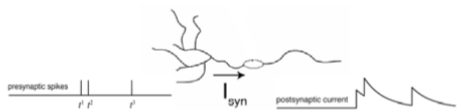
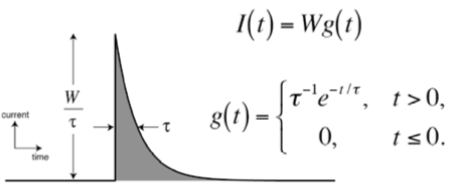
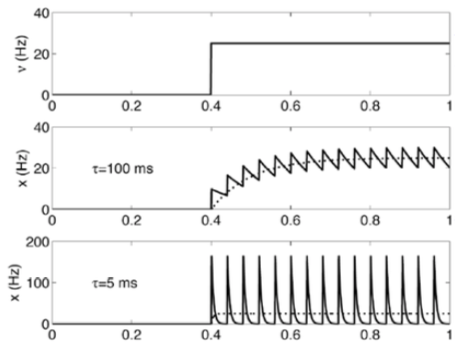
Thus, we can use a quantized leaky integrator model as a basic signal pattern like in Figure16. If the time decay factor τ is large enough, this model is equivalent to classical rate model, which describes a neural activity in terms of continuous variable rate of spiking. The Figure17 shows it clearly.

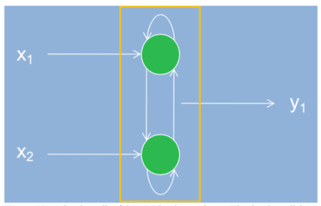
Simple Characteristics of SFNN The SFNN is a quantized leaky integrated model and uses quantum neurodynamics. Also, it adopts a bayesian probabilistic model. Consider it in Figure18.

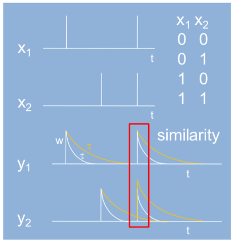
The SFNN always finds a similarity between inputs. The similarity is defined in two different perspectives: inter-similarity and intra-similarity. Whereas the inter-similarity indicates how much similar the current inputs are with the previous ones in temporal comparison, the intra-similarity indicates how much similar the inputs are at a certain time. The Figure18 shows an intra similarity between y1 and y2. The inputs of SFNN are always discrete values, and the outputs of SFNN are energy patterns drawn from calculating similarities, which are Expectation Values of spikes. To train a SFNN, calculate an energy distribution of outputs when a training set is given. If the distribution is not equal to the desired outputs, which is a supervised mode, then calculate new spike probability and adjust it. To get more precise result, I applied Bayesian probabilistic method. Based on these results, calculate new energy distribution and repeat the whole process until the outputs are satisfied. This learning rule is shown in the followings.

• calculate energy distribution
• if not satisfied
  • calculate posterior from prior and likelihood
  • adjust hyperparameters
• calculate new energy distribution
• repeat until satisfied

Because we use quantum neurodynamics, all energy distributions can be represented as binary values, success or failure. Also, current neural state is dependent on the previous spiking states. Thus, to predict the next firing or spike, I used a binomial probability distribution (Bin), which is a discrete probability distribution of the number of successes in a sequence of n independent yes/no experiments, each of which yields success with probability p. The binomial distribution is shown in Figure19.

Applying the binomial distribution to neural activity, we should predict m spikes out of N stimulus with p firing probability. The m and N values are given by training set. But, the firing probability p should be determined by training. The firing probability can change whenever the stimulus is changed. To get right probability, a Bayesian method is introduced. In the Bayesian method, the posterior probability is determined by the prior probability and likelihood function. Because I used a binomial probability distribution as a likelihood function, to get tractable form of calculation, I used a beta distribution, which is conjugates form of prior. The posterior is the product of the prior and likelihood, and becomes also a beta distribution. A typical beta distribution is shown in Figure20.

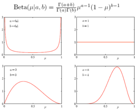
As seen in Figure20, the beta distribution is adjustable by hyperparameters a and b, which can change the probability distribution. In this respect, the learning in SFNN is to find the values of a and b to satisfy the given conditions in the Bayesian paradigm. The posterior probability is like this:

And, the firing probability calculated by the posterior probability is shown here, where l = N – m.

For example, the Figure21 shows a calculation process of the posterior probability distribution graphically. With the prior distribution (left) and likelihood function (middle), the posterior probability can be calculated.

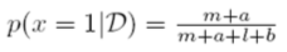
Logical Operations (Example) To find out how much the SFNN works well, I tried to apply it to a simple logical operations, AND and OR. It is so simple that we can implement it with two inputs and one output in Matlab® R2007a environment. The training set is also simple so that it consists of four sample data for each training set. The learning is done in supervised mode, and only one energy distribution is compared. The following Figure22 shows the designed model and the result.

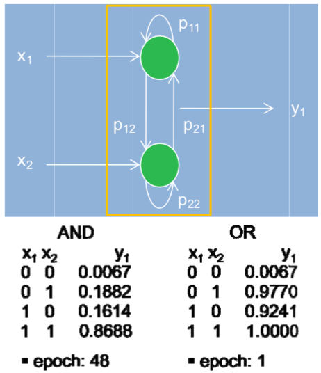
Two synapses are fully connected and their relationship, that is, similarity is evaluated by firing probabilities. There are two types of connections: self-loop and interconnections. The former indicates self-reinforcement effect such as LTP, and the latter indicates inter-synapse effects such as hebbian learning. Sensory to Motor In order to explain the whole brain function, we must show the signal pathway from sensory to motor, which has huge complexity. Using SFNN model, we have a hierarchical model for them. In Figure23, I show new model for brain function which has three distinct levels, in which three SFNNs are used. At each level, the SFNN looks for any similarities between inputs and generates corresponding energy level distributions. The interconnections between two levels consist of two kinds of operations. One is IS-A relation and the other is PART-OF relation. The IS-A connection means a single directed arc and any kinds of information in the previous level or node are transferred to the next level. In this case, the latter is explained with the previous one.

In contrast, the PART-OF connection consists of many directed arcs that are connected to one target node, or vice versa. This means that there is a composition or decomposition of information. Those two conceptual connections are useful to implement systematic functions of brain. In this way, the proposed Scale-Free Neural Network is useful for modeling real brain, as well as implementing artificial intelligence.

DISCUSSION

Though the SFNN has many advantages due to be inspired from biological studies, it still has many open questions. Generalization First of all, it should be generalized to be used widely in industry or brain research. In this work, I simulated it only in case of simple logical operations. To get it, I introduced many biological analogies and statistical method such as Bayesian probability and the learning algorithm is a process of finding hyper-parameters of probabilistic functions. This method is not fully verified and may be limited to only this case. Besides, the nodes of SFNN are fully connected. To achieve real scale-free network, the SFNN can explain the process that one or some hub nodes emerge by calculating the probabilistic functions. This is not clear yet. With all this analysis, the SFNN must have compa- rable or superior performance to the conventional ANNs to be used for both brain research and industrial uses. Thus, various benchmarking works are needed later. Convergence Problem The second issue is convergence problem of SFNN. Training a network is not easy thing, due to its long process. To train the SFNN, I used the error values and stopped training when the error comes within a certain boundary. That is, the probability error difference is the most considerable values here. But, is it really true or plausible? Or, is it really converged? The stopping issue of training is very hard and is to be proved before using it. Therefore, we need to know and prove its plausibility mathematically later. Explanation of real neuron and brain The last issue is the biological or neurological explanation of SFNN. From the beginning, the SFNN is modeled with various biological facts or results, and its main purpose is to study real brain behavior, not industrial application. Therefore, it must be able to explain the real brain behavior and even predict its behavior in specific condition. Though it can’t explain our brain behavior, however, it has at least an industrial application.

ACKNOWLEDGMENTS

I utilized Matlab® R2007a to design an experiment and make a model for the simple logical operation case to verify my idea.

REFERENCES

1. Abeles, M. 1991. Corticonics: Neural Circuits of the Cerebral Cortex, Cambridge Univ. Press.

2. Barabási, A-L. 2003a. Linked, Plume Books.

3. Barabási, A-L. 2003b. Scale-Free Networks, Scientific American.

4. Baylis, G. C. et al. 1985. “Selectivity between faces in the responses of a population of neurons in the cortex in the superior temporal sulcus of the monkey”, Brain Research, pp. 91-102.

5. Bishop, C. M. 2006. Pattern Recognition and Machine Learning, Springer.

6. Clem, R. L. et al. 2008. “On going in vivo experience triggers synaptic metaplasticity in the neocortex”, Science, pp. 101-104.

7. Davison, I. G. and Katz, L. C. 2007. “Sparse and selective odor coding by mitral/tufted neurons in the main olfactory bulb”, J. of Neuroscience, pp. 2091-2101.

8. Dayan, P. and Abbott, L. F. 2005. Theoretical Neuroscience, MIT Press.

9. Hoyer, P. O. 2004. “Non-negative Matrix Factorization with Sparseness Constraints”, J. of Machine Learning Research, pp. 1457-1469.

10. Jain, A. K. et al. 1996. “Artificial Neural Networks: A Tutorial”, Computer, IEEE, pp. 31-44.

11. Kim, D. S. 1995. Neural Networks, HighTech Info Co.

12. Koch, C. 1999. Biophysics of Computation, Oxford Univ. Press.

13. Lee, D. D. and Seung, H. S. 1999. “Learning the parts of objects by non-negative matrix factorization”, Nature, pp. 788-791.

14. Rolls, E. T. et al. 2002. Computational Neuroscience of Vision, Oxford Univ. Press.

15. Seung, H. S. 2006. Lecture Note, MIT Univ.

16. Tsotsos, J. K. 1987. “Representational Axes and Temporal Cooperative Processes”, Arbib, M. A. and Hanson, A. R. eds. Vision, Brain, and Cooperative Computation, pp. 361-417, MIT Press.

17. Vogel, D. D. 1998. “Auto-associative memory produced by disinhibition in a sparsely connected network”, Neural Networks, pp. 897-908.